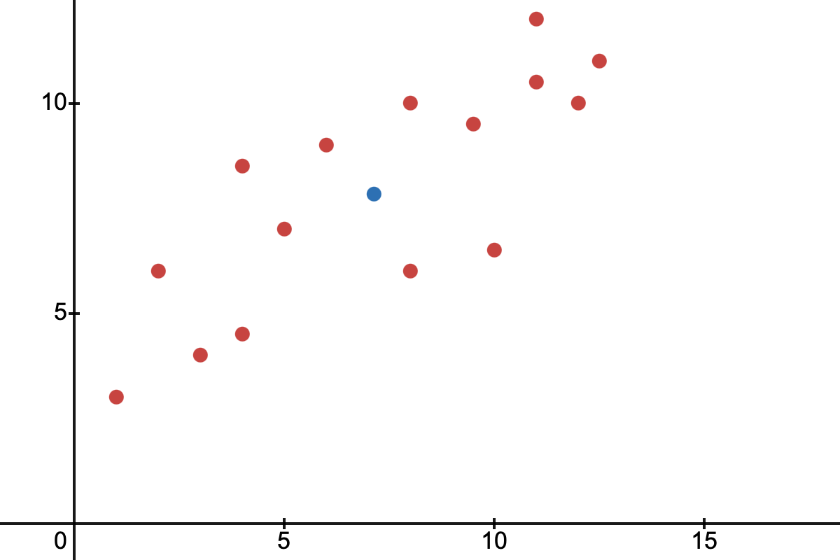
Consider \(n\) data points \((x_i, y_i)\), where \(x_i\) and \(y_i\) are the observed values of \(X\) and \(Y\) on the \(i\)-th trial. The points are shown in this graph along with the mean \((\overline{x}, \overline{y})\) (blue dot):
We want to find a way to measure the correlation. One place we can start is the covariance (\(\operatorname{cov}(X,Y)\)), which takes into account the distance from the mean for both \(X\) and \(Y\):
\(p_i\) is the probability of the data point \((x_i,y_i)\) occurring. For the sake of simplicity, we will assume that all data points have equal chance of occurring:
Why might one use covariance? Let's explain by splitting the plane into four quadrants, one horizontal split along the mean point and a vertical split along the mean point:
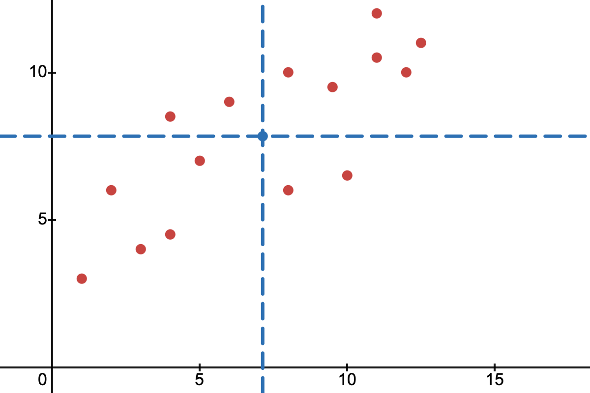
The value \(x_i - \overline{x}\) is the horizontal deviation from the mean of the point \((x_i, y_i)\), while \(y_i - \overline{y}\) is the vertical deviation from the mean of the point \((x_i,y_i)\). If you think about it, \((x_i - \overline{x})(y_i - \overline{y})\) gives the area of a rectangle with width \(x_i - \overline{x}\) and height \(y_i - \overline{y}\):
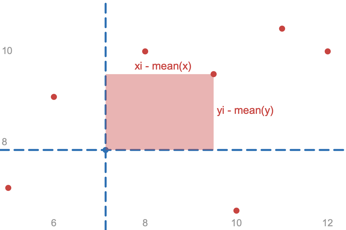
In the top right quadrant, this area would be positive, since both \(x_i - \overline{x}\) and \(y_i - \overline{y}\) are positive. The same can be said about the bottom left quadrant, since both \(x_i - \overline{x}\) and \(y_i - \overline{y}\) are negative. In the top left and bottom right, however, one of the deviation values is negative while the other is positive, this would give negative area:
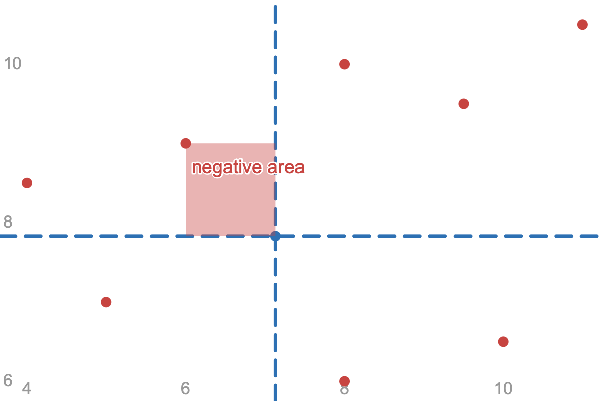
Since \((x_i - \overline{x})(y_i - \overline{y})\) measures signed area, then \(\frac{1}{n} \sum (x_i - \overline{x})(y_i - \overline{y})\) measures the average net area.
If the data is positively correlated, then most of our data points would be in the top right and bottom left quadrant, leading to the positive areas overtaking, resulting in a positive covariance.
If the data is negatively correlated, then most of our data points would be in the top left and bottom right quadrant, leading to the negative areas overtaking, resulting in a negative covariance.
If the data is evenly spread across all four quadrants, the negative areas will cancel out the positive ones, leaving the net area to be around zero.
It seems like covariance is a good measure of correlation. However, there is one problem. Consider another set of data points \((a_i,b_i)\) (green dots) from variables \(A\) and \(B\) that are like \((x_i,y_i)\) but with a smaller variance. Their mean is the same:
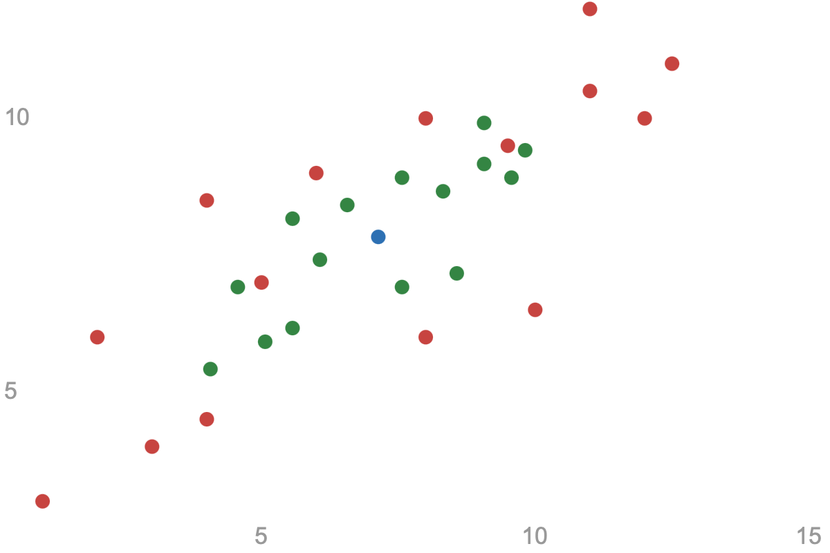
Both of these have the same correlation, but since one of the dataset has a smaller spread, its covariance would also be smaller. This is because there is less deviation from the mean, and therefore the net rectangle areas are smaller. We wish to have a formula which doesn't get affected by the standard deviation. We can achieve this by normalizing the dataset. Instead of using \((x_i,y_i)\), we will use \((w_i,z_i)\), where:
So for now, we will define \(\operatorname{corr}(X,Y)\) as:
We will change the formula if it's not calculating the correlation properly. The formula above removes the standard deviation issue by normalizing the data. This way, \(\operatorname{corr}(X,Y)\) and \(\operatorname{corr}(A,B)\) would have the same value even if they have different standard deviations.
The plot below shows the points \((w_i,z_i)\):
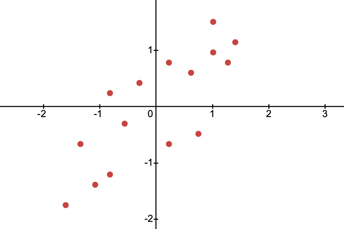
The value \(w_i z_i\) gives the area of rectangle with width \(w_i\) and height \(z_i\):
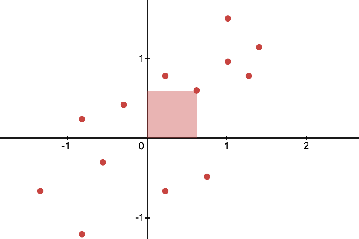
This means \(\frac{1}{n} \sum^n_{i=1}w_i z_i \) gives the average net area. Is this formula a good measure of correlation? Consider the mean of the squared difference between \(w_i\) and \(z_i\):
The average of the sum of squared values is basically variance (when the mean is zero). Since the standard deviation is 1, then so is the variance:
Since a squared variable is always \(\ge 0\):
Similarly:
We found an upper bound and a lower bound for \(\operatorname{mean}(w_i z_i)\). Since \(\operatorname{corr}(X,Y) = \operatorname{mean}(w_i z_i)\):
So far we know a few things about the \(\operatorname{corr}\) function:
- It is bounded between -1 and 1.
- It doesn't change when X or Y is rescaled or shifted.
- The value may be positive, negative or 0 depending on how the data is distributed among the quadrants.
There is one more thing we need to check. With data that is positively correlated, does the \(\operatorname{corr}\) function give a small positive value when the correlation is weak, a large positive value (close to but less than 1) when the correlation is strong, and exactly 1 when the correlation is perfect. For this, we need to go back to the mean squared difference:
Or:
If all the vertical deviations are close to the corresponding horizontal deviations (all the areas are almost a square), then \(\operatorname{mean}((w_i-z_i)^2)\) would be very small, as \(z_i\) would be close to \(w_i\). Keep in mind that \(\operatorname{mean}((w_i-z_i)^2) \ge 0\). If \(\operatorname{mean}((w_i-z_i)^2)\) is close to 0, then \(\operatorname{corr}(X,Y)\) would be close to 1.
In other words, the closer the points are to the diagonal line \(z=w\), the closer \(\operatorname{corr}\) is to 1, and the further the points are from the diagonal line, the further \(\operatorname{corr}\) is from 1.
If all the points are on the diagonal line \(z=-w\), then all of the areas would be squares in the top left and bottom right quadrants (giving negative area). Since they all form a square, then \(z_i = -w_i\):
This shows that if the points were perfectly negatively correlated, then \(\operatorname{corr}\) would be -1, which is the lowest value.
In conclusion, the formula given below can be used for measuring correlation: