Understanding the R^2 score

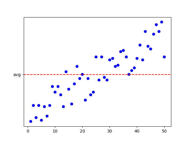
Suppose we are given a set of random data:

\[ y_1, y_2, \ldots, y_n \]

Assuming you know nothing about what influences \(y_i\), what is the best way to predict future values of \(y_i\)? A convention is to use the average (\(\overline{y}\)). Assuming the future will mirror the overall historical baseline by taking the mean of all past data. It works best for stable data with no strong trends.

Upon studying more about \(y_i\), you realize that it is influenced by \(x_i\).

\[ \begin{gather} y_1, y_2, \ldots, y_n \\ x_1, x_2, \ldots, x_n \end{gather} \]

If you want to guess what \(y_{n+1}\) would be, a naive approach would be to use the average value (\(y_{n+1} = \overline{y}\)).

We can use the regression line here. But now the question is, how good is our regression line compared to the average (assuming we're using OLS)? If \(x_i\) and \(y_i\) had little to no correlation, then using a regression line would be no better than using the average. However with a strong correlation, the regression line should perform much better than the baseline:

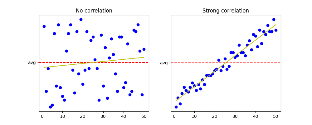
We can compare the regression line and the baseline by comparing the sum of squared residuals and the total sum of squares. The sum of squared residuals (SSR) is the sum of the squares of the difference between the observed value and the estimated value: \(\sum (y_i - \hat{y_i})^2 \). The total sum of squares (SST) the sum over all squared differences between the observations and the mean: \(\sum (y_i - \overline{y})^2\). We can use this to measure how much better the regression line is:

\[ \frac{\sum (y_i - \hat{y_i})^2}{\sum (y_i - \overline{y})^2} \]

If there is a perfect correlation, then the regression line would perfectly fit our data points, then \(y_i - \hat{y_i} = 0\) for all \(i\), which means the above fraction would be 0. If there is a very poor correlation, then SSR would be very close to SST. Keep in mind that since the OLS regression line finds the estimation line which minimizes the sum of squared residuals, then SSR would always be less than SST, which means:

\[ 0 \le \frac{\sum (y_i - \hat{y_i})^2}{\sum (y_i - \overline{y})^2} \le 1\]

This means if the fraction is closer to 1, then our regression line is no better than simply using the average, and if the fraction is closer to 0, then our regression line is significantly better. The \(R^2\) score uses this but the 1 and 0 flipped:

\[ R^2 = 1- \frac{\sum (y_i - \hat{y_i})^2}{\sum (y_i - \overline{y})^2} \]

If we use the \(R^2\) score, then a number closer to 1 is a good score, while a number closer to 0 is a bad score. The \(R^2\) score for the first graph is 0.81.

Understanding the R² score